
Little Snake River near Lily, CO
The White River and Yampa River (with its main tributary, the Little Snake River) together contribute about 15% of the flow of the Upper Colorado River Basin.With relatively few dams and diversions, they have a largely unimpaired flow regime and provide regionally important habitat for native fish, including the four endangered species in the Upper Colorado River Basin. The White and Yampa Rivers also comprise nearly all of the streamflow within the state of Colorado that is still unappropriated and legally available for consumptive use. Thus, these rivers are increasingly attractive to those seeking new water supplies, to serve both urban water use on Colorado's Front Range and energy development on the Western Slope.
Steve Gray, with Jeff Lukas and Connie Woodhouse, used a network of existing tree-ring chronologies to generate streamflow reconstructions for the White River, the Yampa River, and the Little Snake River (Gray et al. 2011). The Little Snake River near Lily, CO, gage, represents the flow of the Little Snake River just before it joins the Yampa River.
References:
Gray, S. T., J. J. Lukas, C. A. Woodhouse. 2011. Millennial-length records of streamflow from three major upper Colorado River tributaries. Journal of the American Water Resources Association, 47(4): 704-712. DOI: 10.1111/j.1752-1688.2011.00535.x. (Abstract)
Methods
The original pool of 67 predictors (tree-ring chronologies from Colorado, Wyoming, and Utah) was reduced via a series of correlation analyses. First, the observed flow record for the period 1906 to 1997 was compared with tree-ring values. Chronologies with r > 0.5 (p < 0.001) were then subjected to correlation tests over half-sample subsets. Only chronologies with r > 0.5 over the full and r > 0.4 over both the early (1906 to 1951) and late (1952 to 1997) periods were allowed into the final predictor pool.
The reconstruction model was selected from the final predictor pool using a forward stepwise regression approach, calibrated on the observed flows from 1906-2001. Briefly, predictors enter or leave the model based on F-level, which must show p < 0.05. To avoid over-fitting, the stepwise process was stopped when the root mean square error (RMSE; Weisberg, 1980) was not reduced by the entry of additional predictors. Variance inflation factor and Mallow's Cp were also used to test for multicollinearity of the predictors.
The final reconstruction presented here is a composite generated from two models: one including the Pumphouse chronology, which extends back to 1315, and one without Pumphouse, which extends further back but has a slightly poorer fit to the observed flow record (see below). The no-Pumphouse model was used to generate the values from 1000-1314, while the with-Pumphouse model was used to generate the values from 1315-2002. The variance in the pre-1315 portion of the record was rescaled to match the variance in the post-1315 reconstruction.
(Note: Linear regression modeling, when the y-intercept is modeled as negative, can generate negative annual flow values, such as the reconstructed -10 KAF flow in 1460. The uncertainty around the reconstructed value for 1460 does include positive flow values that are more physically plausible.)
The standard chronologies, containing low-order persistence as found in the underlying tree-ring data, were used. Four predictor chronologies were selected by the stepwise procedure for the reconstruction model. Validation statistics were computed using a leave-one-out (cross-validation) approach.
Predictor Chronologies: Trail Gulch (CO), Wells Draw (UT), Encampment (WY) Pumphouse (CO)
| 1000-1314 model Statistic | Calibration | Validation |
| Explained variance (R2) | 0.58 | |
| Reduction of Error (RE) | 0.55 |
| 1315-2002 model Statistic | Calibration | Validation |
| Explained variance (R2) | 0.61 | |
| Reduction of Error (RE) | 0.57 |
(For explanations of these statistics, see this document (PDF), and also the Reconstruction Case Study page.)
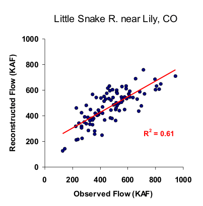
Figure 1. Scatter plot of observed and reconstructed Little Snake River annual flow, 1906-2001.
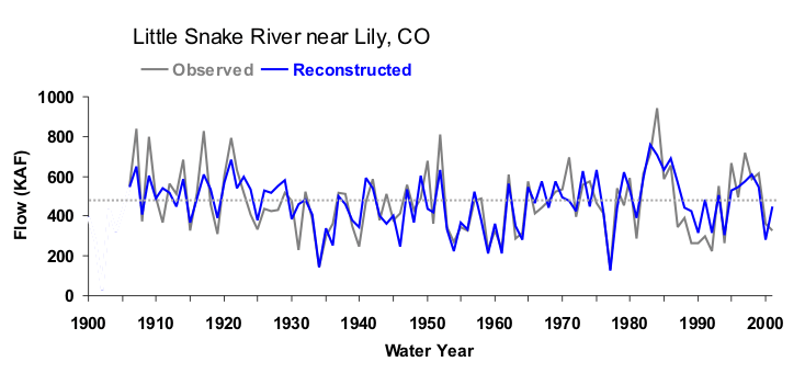
Figure 2. Observed (black) and reconstructed (blue) annual Little Snake River annual flow, 1906-2001. The observed mean is shown by the dashed line.
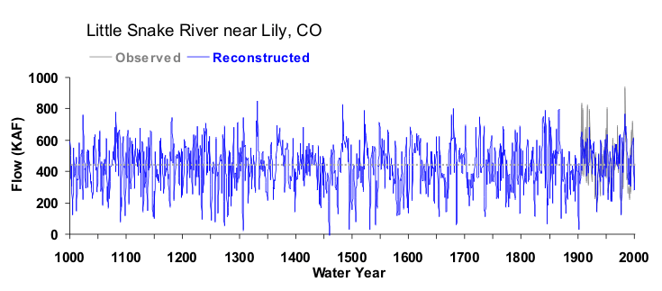
Figure 3. Reconstructed annual flow for the Little Snake River (996-2001) is shown in blue. Observed flow is shown in gray and the long-term reconstructed mean is shown by the dashed line.
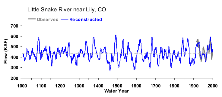
Figure 4. The 10-year running mean (plotted on final year) of reconstructed annual flow for the Little Snake River, 996-2001. Reconstructed values are shown in blue and observed values are shown in gray. The long-term reconstructed mean is shown by the dashed line.